Evaluating the Water Quality Benefits of a Bioswale in Brunswick County, North Carolina (NC), USA

Abstract

Standard roadside vegetated swales often do not provide consistent pollutant removal. To increase infiltration and pollutant removal, bioswales are designed with an underlying soil media and an underdrain. However, there are little data on the ability of these stormwater control measures (SCMs) to reduce pollutant concentrations. A bioswale treating road runoff was monitored, with volume-proportional, composite stormwater runoff samples taken for the inlet, overflow, and underdrain outflow. Samples were tested for total suspended solids (TSS), total volatile suspended solids (VSS), enterococcus, E. coli, and turbidity. Underdrain flow was significantly cleaner than untreated road runoff for all monitored pollutants. As expected, the water quality of overflow was not significantly improved, since little to no interaction with soils occurred for this portion of the water balance. However, overflow bacteria concentrations were similar to those from the underdrain perhaps due to a first flush of bacteria which was treated by the soil media. For all sampling locations, enterococci concentrations were always higher than the USEPA geometric mean recommendation of 35 Most Probable Number (MPN)/100 mL, but there were events where the fecal coliform concentrations was below the USEPA’s 200 MPN/100 mL limit. A reduction in TSS concentration was seen for both overflow and underdrain flow, and only the underdrain effluent concentrations were below the North Carolina’s high quality water limit of 20 mg/L. Comparing results herein to standard swales, the bioswale has the potential to provide greater treatment and become a popular tool.

1. Introduction

Urbanization is a global trend, with 54% of the total population living in urban areas in 2014 and expected to reach 66% by 2050 [1]. Urbanization negatively impacts the environment, notably water quality, due to an increase in impervious cover [2,3,4,5,6]. Urban runoff contains pollutants including suspended solids, heavy metals, nutrients, and pathogens [7,8,9]. Pathogens have been reported as one of the leading causes for impaired surface waters placed by the United States Environmental Protection Agency (USEPA) [10]. Elevated bacteria levels can lead to economic losses in recreation waters, increased drinking water treatment costs, and potential health concerns [11].

There are many external factors impacting the fate of bacteria in a watershed including: a variety of sources (domestic pets, wild birds and animals, and human waste) [12] and various environmental factors (temperature, light intensity, and predation) [13,14,15,16], and treatment within stormwater control measures (SCMs). Removal mechanisms for bacteria include filtration, adsorption to a soil, desiccation, and predation [14]. Biofilm development may enhance adsorption to a soil [17,18]. However, bacteria can be difficult to permanently sequester, due to the potential to reproduce in a soil [13,19].

Little research is available regarding whether bioretention media promotes bacterial sequestration or provides an environment for growth [20]; through growth and resuspension, media could act as a source of bacteria to stormwater runoff. While ‘true’ pathogens are the biggest concern, fecal indicator bacteria (FIB) are the regulatory metric used to monitor water quality and public health decision making [21,22,23,24]. Fecal indicator bacteria (FIB) include Escherichia coli (E. coli), enterococci, and total and fecal coliforms [16]. While not pathogenic, FIB are associated with fecal matter, thus signaling the potential presence of human pathogens [25]. In addition, FIB are usually found in higher numbers, have a higher survival rate, and are easier and more economical to detect in laboratory testing than true pathogens [26,27]. Understanding how unit processes (for FIB and pathogens) can be employed in SCMs is integral to reducing the impacts of bacteria in stormwater on receiving waters.

Stormwater runoff can be managed using low-impact development (LID) techniques, which targets treatment of a water quality volume at or near the source of runoff [28]. LID techniques attempt to mimic the hydrologic and water quality characteristics of the pre-development watershed [29,30].

One commonly installed LID SCM is a bioretention cell (BRC). Pollutant removal is primarily reliant on the engineered bioretention media, which is generally sand-based with small amounts of silt, clay, and organic matter [31]. The goal of a BRC is to reduce stormwater runoff volume, control peak flows, and improve water quality through filtration, infiltration, and nutrient transformation [31].

Dry swales are shallow, vegetated channels that are generally designed and constructed with a triangular or trapezoidal cross-section and are typically for stormwater conveyance [32,33]. Dry swales have reported mean volume reduction from 23 to 47% [29,34,35,36,37,38], which translates into pollutant load reduction for receiving waters [29,31,38]. Pollutant removal mechanisms employed by standard swales include: sedimentation, filtration, infiltration, and modest amounts of biological and chemical reactions at the soil surface [32,39,40]. Although there is growing literature on the capabilities of swales to reduce runoff [32,38,39,40,41], a lack of consistent water quality treatment has been observed in dry swales, in particular for bacteria removal [25,42].

Bioswales are a category of SCM which combine the conveyance function of a traditional grass swale with the filtration and biological treatment mechanisms of bioretention [43]. While similar in appearance to a grassed swale, a bioswale employs an engineered soil media, similar to bioretention media, below the vegetation; the media is underlain by a gravel drainage layer surrounding a perforated underdrain. A bioswale promotes infiltration and filtration through the largely-sand media and underdrain while maintaining stormwater conveyance on the surface during large rainfall events. Natural organic material (NOM) is included in the media mixture to promote chemical transformations and sorption of phosphorus and heavy metals [44,45]. Only a few studies of FIB removal through soil media have been conducted, most of which show up to 1-log reduction in FIB concentrations. Rusciano and Obropta [18] found a 91.5% removal of fecal coliform bacteria through bio-media columns, Garbrecht et al. [46] found E. coli reduction coefficients between 32–91% based on the soil type in the column, and Hunt et al. [47] found an average of 69% and 71% removal of fecal coliform and E. coli, respectively, from stormwater runoff treated by a bioretention cell. However, virtually no data exist on the performance of bioswales for runoff conveyance, water quality treatment, or bacteria removal capabilities [25,48,49,50].

While preliminary research on bioswales does show the potential for stormwater runoff volume reduction [51,52,53], the exact extent of this reduction is not well known. Research is needed to determine how incorporating soil media and an underdrain affect volume reduction and how their pollutant removal mechanisms affect bacteria sequestration and subsequent removal.

2. Materials and Methods

2.1. Lumber River Basin and Lockwoods Folly River Description

The study site was located in Bolivia, North Carolina (NC) in Brunswick County (34°0′16.2972″ N, 78°15′38.7792″ W) and drains into the Lockwoods Folly River, which is located in the Lumber River Basin. Pathogens, nutrients, and sediment loads were all problems in this watershed [54]. High levels of fecal coliform bacteria have caused the Lockwoods Folly River to be included in the USEPA’s 303(d) list of impaired waters and have resulted in its closure to shellfishing [55]. The stressors of urbanization are expected to exacerbate these problems as Brunswick County, NC, is the 31st fastest growing county in the United States during 2010–2016 [56].

2.2. Brunswick County Bioswale

2.2.1. Watershed Characteristics

To treat road runoff, a bioswale was installed in the right-of-way on NC 211, approximately 1.6 km east of its intersection with US17. NC 211 is a two-lane state highway with an asphalt wearing course which was in good condition during the study period. The drainage area was 0.74 hectares, 44% of which was directly connected impervious area. Pervious areas were the existing grassed shoulders, in good condition and on a 4:1 horizontal distance:vertical distance (H:V) slope with highly transmissive, sandy soils. Diffuse stormwater runoff from the northern lane of the two-lane road discharged directly onto the grass shoulder, which acts as a vegetated filter strip, allowing for initial settling of sediment and particulate-borne contaminants and for some infiltration. A portion of this channel was removed to install the forebay and bioswale. The concrete-lined channel first drained into a forebay (Figure 1), which served to dissipate energy and prevent erosion in the bioswale. The bioswale commenced immediately downslope of the forebay.

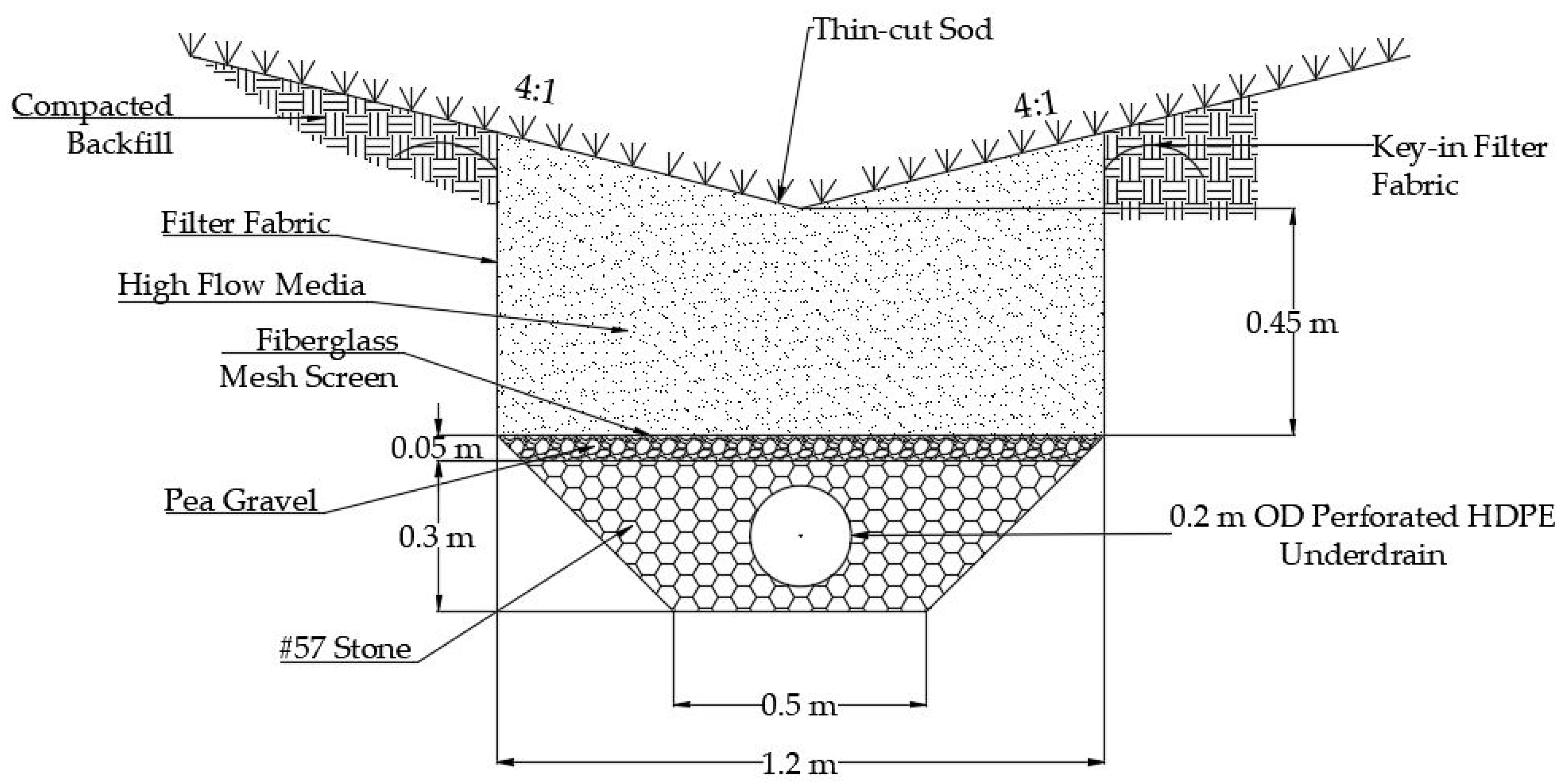
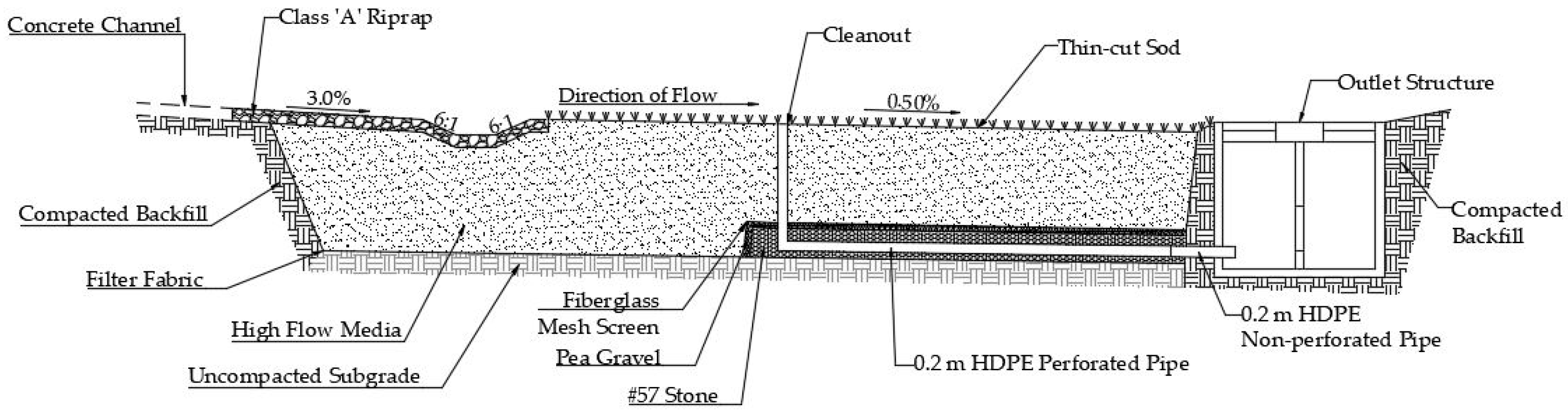
2.2.2. Bioswale Design

The forebay is 2.7 m wide by 10.7 m long. The initial 6.1 m was a triangular channel on a 3% slope. The plunge pool consisted of the latter 4.6 m of the forebay and has a depth of approximately 0.15 m. The slope into and out of the pool was 6:1 (H:V). The entire forebay was lined with class A rip-rap (50 to 150 mm diameter stone [57]) to a depth of 0.2 m. The high flow media (

Table 1. High flow media characteristics.

Characteristic	Value
Hydraulic conductivity (Ksat)	2540 mm h−1
Peat Moss	15% by volume
Total Carbon	>85%
Carbon to Nitrogen Ratio	15:1 to 23:1
Lignin Content	49–52%
Humic Acid	>18%
pH	6.0–7.0
Moisture Content	30–50%
Passing 2.0 mm sieve	95–100%
Passing 1.0 mm sieve	>80%
Sand-Fine	<5%
Sand-Medium	10–15%
Sand-Coarse	15–25%
Sand-Very Coarse	40–45%
Gravel	10–20%
Clay/Silts	<2%

), approximately 0.9 m deep, began 1.8 m past the start of the rip-rap lined channel and continued under the forebay to ensure that the system completely drained inter-event.

To create the bioswale, a trench with a width of 1.2 m, depth of 0.8 m, and length of 30.5 m was excavated, starting at the end of the plunge pool. Once excavated, the entire trench, including under the rip-rap channel and plunge pool, was lined with a high flow fabric prior to being backfilled. This fabric ensured the high flow media remained within the system, but allowed water that passed through the media to infiltrate into the underlying soil. The first 11 m, starting at the end of the plunge pool, was completely (all 0.9 m) filled with only the high flow media.

After the first 11 m, a perforated underdrain was installed. The trapezoidal base of the ditch was filled with a 5 cm layer of ASTM standard #57 stone (2.36 to 37.5 mm stone size [58]), serving as internal water storage (IWS), which has been shown to substantially improve runoff reduction within bioretention cells by promoting inter-event exfiltration [59,60]. Then, 18 m of perforated high-density polyethylene pipe (HDPE) pipe (0.2 m diameter) (Advanced Drainage Systems, Inc., Raleigh, NC, USA) was placed over the stone layer, creating an IWS zone of 5 cm. The pipe was covered with 5 cm ASTM #57 stone. Next, a pea gravel layer was placed on top of the ASTM #57 stone. Finally, a fiberglass mesh screen was placed around the pea gravel (Figure 2). These ‘choking’ layers of gravel and media limited soil media movement to the underdrain. The remaining trench volume was filled with the high flow media and covered with a thin-cut warm-season sod. The resulting bioswale consisted of a triangular channel with 4:1 H:V side slopes and a total length of 42 m. A longitudinal cross-section of the full bioswale system can be seen in Figure 3, with design characteristics in

Table 2. Bioswale design characteristics.

Characteristic	Value
Rip-rap channel length	6 m
Rip-rap channel slope	3%
Plunge pool length	4.6 m
Plunge pool depth	0.15 m
Underdrain length	18.3 m
Underdrain diameter	0.2 m
Media depth	0.45–0.9 m
Total length	42 m
Surface geometry	Triangular
Surface side slopes	4:1
Media void storage	22.7 m3
Surface storage	14.2 m3

.

The bioswale underdrain and surface flow discharged into the existing outlet structure (Figure 4). The first chamber housed the monitoring equipment for the underdrain; surface flow was prevented from mixing with underdrainage. Bioswale overflow was monitored in the downstream chamber. The outlet structure was elevated 15 cm above the swale, resulting in up to 67% of the bioswale surface area being inundated during a storm. The maximum cumulative storage within the bioswale at the brink of overflow was 36.9 m³, 14.2 m³ of surface storage and 22.7 m³ of soil void space.

2.2.3. Climatic and Water Quality Data Collection

As stormwater entered the bioswale (rip-rap), a wooden board was used to pool water for sample aliquot collection. Inlet aliquots were collected using a Teledyne ISCO 6712 (Lincoln, NE, USA) automated sampler. Sampling was triggered by two nearby rain gauges, the first enabled the sampler after 2.54 mm of rainfall had occurred, while the second triggered the sampler to obtain 200 mL aliquots after each additional 1 mm of rainfall. Thus, the maximum rainfall depth which could be sampled was 52 mm. However, the 1-mm trigger was increased in anticipation of several larger storm events, and the actual maximum rainfall depth for a sampled storm event was 92 mm Since rainfall depth is considered a good predictor of runoff volume in urbanized watersheds, these samples were considered flow-proportional [61].

At the underdrain and overflow monitoring points in the outlet structure, purpose-built weirs were installed to measure discharge with time. Each weir had an ISCO 6712 automated sampler with a 730 bubbler module, which measured flow depth over the weir plate (Figure 5). The sampler converted the flow depth to a corresponding flow rate using the following equations.

The equation for the 60° underdrain weir is as follows:

$$Q=796.7\times H^{2.5}$$

(1)

where Q is the flow rate in L s⁻¹ and H is the flow depth in m.

The equation for the 90° overflow weir is as follows:

$$Q=1380\times H^{2.5}$$

(2)

where Q is the flow rate in L s⁻¹ and H is the flow depth in m.

Flow rate data at these two monitoring points were integrated with time to determine runoff volume passing each weir on 2-min intervals Equation (3). Automated samplers then obtained volume-proportional 200 mL aliquots on pre-programmed intervals (e.g., every 500 L) throughout the hydrograph. The sample tubing was installed behind the weir plate to ensure samples were collected before overflowing the weir.

$$V=Q\times t$$

(3)

where V is the corresponding volume in L, Q is the corresponding flow rate in L s⁻¹, and t is the time step of 120 s (2 min) sampling interval.

Samples were triggered across the hydrograph based on volume passing over the weir and represented, at minimum, 80% of the total flow volume, characterizing (essentially) the entire pollutograph. Composite samples were analyzed for water quality only if paired inlet and outlet samples were obtained.

The rainfall depth in the on-site manual rain gauge was checked during each sampling mission to compare against the tipping bucket rain gauge data. Rainfall and water quality data were collected over a 1-year period (25 February 2014 through 26 February 2015).

2.3. Water Quality Analysis

Stormwater runoff samples were obtained from the ISCO samplers within 24 h of the cessation of rainfall. The 10 L composite sample bottles were shaken vigorously to re-suspend sediment and sub-sampled into laboratory containers for transit. The remaining sample volume in the composite sample jar was discarded and the bottle washed with deionized water and replaced within the ISCO sampler for the next storm event. Samples were placed on ice immediately after sub-sampling and chilled to less than 4 °C for transit to the Environmental Quality Laboratory at Coastal Carolina University. All samples were measured for conductivity, turbidity, total suspended solids (TSS), volatile suspended solids (VSS), enterococci (Ent), and fecal coliform (FC) using Standard Methods [62,63,64,65,66] except enterococci [67] Lab duplicates and field duplicates were analyzed for all water quality parameters (TSS, turbidity, VSS, fecal coliform, and enterococci) for the inlet sample, because this was the location with the largest collected sample volume. All duplicates were within 20% relative percent difference.

2.4. Statistical Analysis

The water quality data were statistically analyzed to compare paired influent and effluent water quality for five parameters: TSS, turbidity, VSS, fecal coliform, and enterococci. Each data set was tested for normality using the Anderson-Darling procedure using α = 0.05. For all water quality parameters, at least one data set (either inlet, underdrain, or overflow) was not normally distributed and was unable to be transformed using log or squared transformations. Kendall’s tau non-parametric rank correlation, therefore, determined statistically significant correlations between pollutants. Tests were also run to determine any correlations between runoff flow concentrations (inflow, underdrain, and overflow) and rainfall characteristics (rainfall depth and antecedent dry period). To assess the effects of treatment, or lack thereof, in the filter media, statistical comparisons, using Wilcoxon Signed Rank Test, were made between the inlet and underdrain and inlet and overflow data sets. A criterion of 95% confidence (α = 0.05) was used for all tests. Statistical analyses were performed using the R software (v. 3.4.3) (R Core Team, Vienna, Austria) [68].

Concentration reductions (CR) were calculated Equation (4) for each pollutant and outlet monitoring point using USEPA’s efficiency ratio [69]:

$$CR=\left(1-\frac{mean outlet concentration}{mean inlet concentration}\right)\ast 100\%$$

(4)

The geometric mean was used for enterococci and fecal coliform; the arithmetic mean was used for TSS, VSS, and turbidity.

Probability plots for enterococci and fecal coliform were created to evaluate the bioswale across all influent and outflow concentrations. The probability was calculated using Equation (5):

$$P=\frac{i-0.5}{n}$$

(5)

where P is the probability of an observation, i is the rank of the observation, and n is the number of observations in the data set [70].

3. Results and Discussion

3.1. Storm Event Characteristics

A total of 15 storm events were sampled for water quality. These storms ranged in rainfall depth from 13.2 to 91.7 mm (mean 38.1 mm), with an antecedent dry period (ADP) from 0.35 to 7.8 days (mean 4.92 days) (

Table 3. Rainfall characteristics for each storm sampling event.

Storm Sampling Event	Date	Rainfall Depth (mm)	Antecedent Dry Period (days)	Sampled for Inlet Flow?	Sampled for Underdrain Flow?	Sampled for Overflow?
1	4/16/2014	18.0	0.35	B, S, T	B, S, T	-
2	5/16/2014	90.9	MD	B, S, T	B, S, T	-
3	6/21/2014	34.0	7.07	B, S, T	B, S, t	-
4	6/24/2014	18.8	1.39	B, S, T	B, S, T	-
5	7/4/2014	69.3	4.56	B, S, T	B, S, T	B, S, T
6	7/25/2014	40.1	MD	B, S, T	B, S, T	B, S, T
7	9/6/2014	25.4	6.79	B, S, T	B, S, T	-
8	9/30/2014	13.2	3.34	B, T	B, T	B, T
9	11/1/2014	25.4	MD	B, S, T	B, S, T	B, T
10	11/23/2014	54.6	6.44	B, S, T	B, S, T	B, S, T
11	1/12/2015	22.9	7.80	B, S, T	B, S, T	B, T
12	1/24/2015	91.7	5.19	B, S, T	B, S, T	B, S, T
13	2/17/2015	17.3	6.23	B, S, T	B, S, T	-
14	2/23/2015	16.5	MD	B, S, T	B, S, T	B, T
15	2/26/2015	33.0	MD	B, S, T	B, S, T	B, S, T

MD: missing datasets, unable to calculate antecedent dry period; B: bacteria (fecal coliform, enterococcus); S: sediment (TSS, VSS); T: turbidity.

). Sampled storm events were collected throughout the year, with 3–4 events captured in each season. However, not all events had enough runoff volume, overflow in particular, to be analyzed for all contaminants (Table 3).

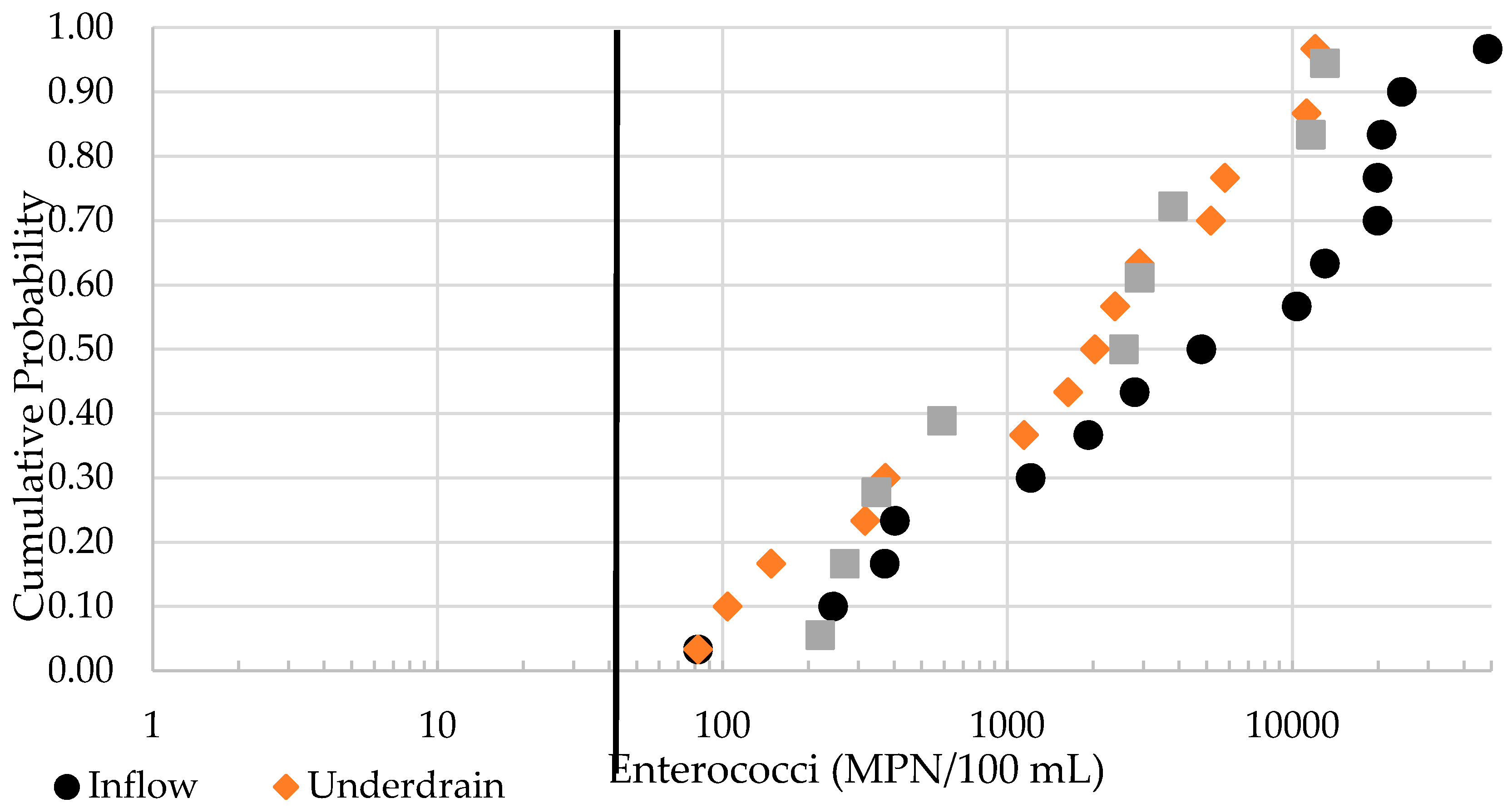
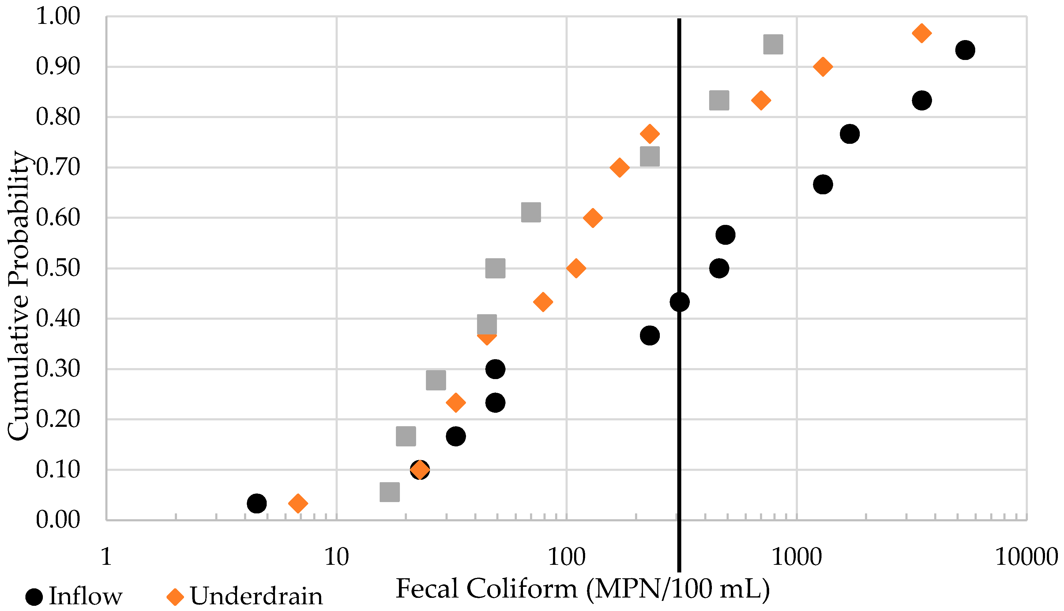
3.2. Impact on Pathogen Indicator Species and Sediment Removal

Non-parametric statistical tests between the runoff concentrations at all monitoring points and the storm characteristics of rainfall depth and antecedent dry period found only two significant correlations (a = 0.05). The positive correlations were between rainfall depth and underdrain VSS concentration (p = 0.043) and rainfall depth and overflow fecal coliform concentration (p = 0.012). These results highlight the complexity of basing the bioswale’s performance on the storm characteristics of rainfall depth and antecedent dry period.

Outflow concentrations for all five pollutants examined were lower, but statistically significant reductions were only observed when comparing underdrain to influent concentrations (

Table 4. Means for pathogen indicator species and sediments and water quality standards.

Sampling Location	Enterococci 1 (MPN/100 mL)	Fecal Coliform 1 (MPN/100 mL)	TSS 2 (mg/L)	VSS 2 (mg/L)	Turbidity 2 (NTU)
Inflow	3451 {903}	320 {126}	35.1 {1.9}	12.4 {0.6}	23.3 {0.5}
Underdrain	1411 (0.004) {290}	111 (0.021) {61}	4.2 (0.000) {0.2}	1.6 (0.000) {0.04}	14.8 (0.000) {0.3}
Overflow	1549 (0.455) {549}	79 (0.180) {30}	31.6 (0.313) {4.7}	9.7 (0.313) {1.3}	22.4 (0.326) {1.3}
North Carolina Limits	35 a	200 b	20.0 b	-	50.0 b

¹ Geometric mean, ² Arithmetic mean, ^a [11], ^b [75], Bolded values were significant reductions with respect to inflow concentrations, italicized values were below the U.S. EPA limits, (p-value compared to inflow concentration), {standard error of mean}.

). A principal pollutant removal mechanism of a bioswale is filtration [71,72], which explains why TSS and VSS concentrations from underdrains were very low (4.2 and 1.6 mg/L, respectively). There was less impact observed in overflow since it does not undergo filtration through the media. However, the bioswale’s forebay and vegetation aids in reducing the runoff velocity, allowing for sedimentation [35,73], thus (non-significantly) reducing TSS concentrations in overflow to 32 mg/L compared to 35 mg/L influent. Overflow results herein can be compared to those of other ‘standard’ swales and were similar, which ranged from 8–70 mg/L TSS [32,35,73,74].

The bioswale reduced fecal coliform concentrations to values less than the U.S. EPA water quality limit of 200 Most Probable Number (MPN)/100 mL [75], but was unable to meet the enterococci swimming limit of 35 MPN/100 mL [11] (

Table 5. Percent reduction of mean from inlet for each pollutant from surface and underdrain samples.

Sampling Location	Enterococci 1	Fecal Coliform 1	TSS 2	VSS 2	Turbidity 2
Underdrain	59%	65%	88%	87%	36%
Overflow	55%	75%	10%	21%	4%

¹ Geometric mean, ² Arithmetic mean, Bolded values were significant reductions.

). However, influent concentrations were 100-fold higher than the federal standards for enterococci and only 1.5 times higher for fecal coliform. Both inflow and outflow also met state standards for turbidity (50 Nephelometric Turbidity Units (NTU)). Underdrain TSS concentrations (mean 4 mg/L) were less than typical water quality standards (20 mg/L), but those of overflow (32 mg/L) were not.

The largest concentration reductions were observed for underdrain TSS (88%) and VSS (87%) because these pollutants were presumably filtered by the fill media (Table 5). Sediment trapping efficiencies were similar to those for bioretention [47] and Austin sand filters [76]. Reductions from inflow to (non-filtered) overflow for these two pollutants were much lower (10% for TSS and 21% for VSS), suggesting water exceeding a bioswale’s capacity for filtration will receive little treatment. Results associated with turbidity were similar albeit influent turbidity was already quite low (23 NTUs); a more noticeable reduction in turbidity was associated with filtered underdrain discharges. Both fecal coliform and enterococci reductions were substantial (>50%) for both underdrain and overflow monitoring points. However, only underdrain effluent was significantly improved compared to influent, perhaps due to the small sample size (n = 5) for the overflow monitoring point.

Figure 6 illustrates that for all storms sampled and at all sampling locations, concentrations of enterococci exceeded the water quality standard of 35 MPN/100 mL. However, approximately 33% of inflow concentrations, 67% of overflow concentrations, and 73% of underdrain concentrations were less than the 200 MPN/100 mL water quality standard for fecal coliform (Figure 7). Up to 1-log difference in fecal coliform at the inlet compared to the underdrain and overflow was observed, supporting the significant treatment of fecal coliform within the bioswale. One interesting finding is that for both enterococci and fecal coliform, the distributions of underdrain and overflow concentrations were quite similar (Figure 6 and Figure 7). One plausible explanation is that bacteria in this study were mobilized primarily during the first flush [77]. Overflow occurs only after the rainfall exceeds the bioswale’s soil and surface storage capacity. When overflow begins, a substantial portion of the bacteria may thus have already been settled and/or filtered out by the soil media (i.e., cleaner inflow at the time overflow begins). While overflow is not treated to the same extent as underdrain flow, lower bacterial concentrations in stormwater runoff after the ‘dirtiest’ water has been mobilized from the watershed may have resulted in similar distributions of underdrain and overflow FIB concentrations.

Results demonstrate the complexities associated with (1) understanding bioswale treatment and (2) determining whether an SCM, including a bioswale, is a ‘good’ practice for FIB treatment. While no previously peer-reviewed studies have reported how a bioswale impacts pollutants, many studies have evaluated the effectiveness of other filtration-based SCMs, in particular bioretention. Taken cumulatively, studies illustrate a wide range of concentration “reductions” for enterococci, fecal coliform, and TSS for various SCMs (

Table 6. Summary of studies reporting bacteria and sediment concentration reductions from SCMs.

Author	Location	SCM Type	Ent.	FC	TSS
			CR	CR	CR
			(%)	(%)	(%)
Herein	Brunswick County, NC	Bioswale Overflow	55	75	10
		Bioswale Underdrain	59	65	88
Hathaway and Hunt [78]	Wilmington, NC	Bioretention cell	89	-	-
		Bioretention cell	−1	-	-
Passeport et al. [79]	Alamance County, NC	Bioretention cell	-	95	-
		Bioretention cell	-	85	-
Davis [80]	College Park, MD	Bioretention cell	-	-	47 a
		Bioretention cell	-	-	62 a
Hunt et al. [47]	Charlotte, NC	Bioretention cell	-	69 a	60 a
Hathaway and Hunt [78]	Wilmington, NC	Wet pond	90	-	-
		Wet pond	87	-	-
Hathaway and Hunt [78]	Wilmington, NC	Wetland	69	-	-
		Wetland	41	-	-
Davies and Bavor [81]	Sydney, Australia	Wetland	85	-	-
Krometis et al. [82]	Central NC	Wet Retention Pond	−108	−41	-
		Wet Retention Pond	36	31	-
Mallin et al. [83]	New Hanover County, NC	Wet Detention Pond	-	86 a	65 a
		Wet Detention Pond	-	56 a	−37 a
		Wet Detention Pond	-	−15 a	−22 a

Ent. CR: Enterococci concentration reduction; FC CR: Fecal coliform concentration reduction; TSS CR: Total suspended sediment concentration reduction; ^a Concentration reduction (CR) manually calculated based on concentrations provided by corresponding author(s).

). The bioswale concentrations herein (particularly those of the filtered effluent from the underdrain) were in the range of or modestly higher than those of other SCMs. Thus, bioswales appear capable of achieving similar results to that of other more commonly-employed SCMs, such as bioretention.

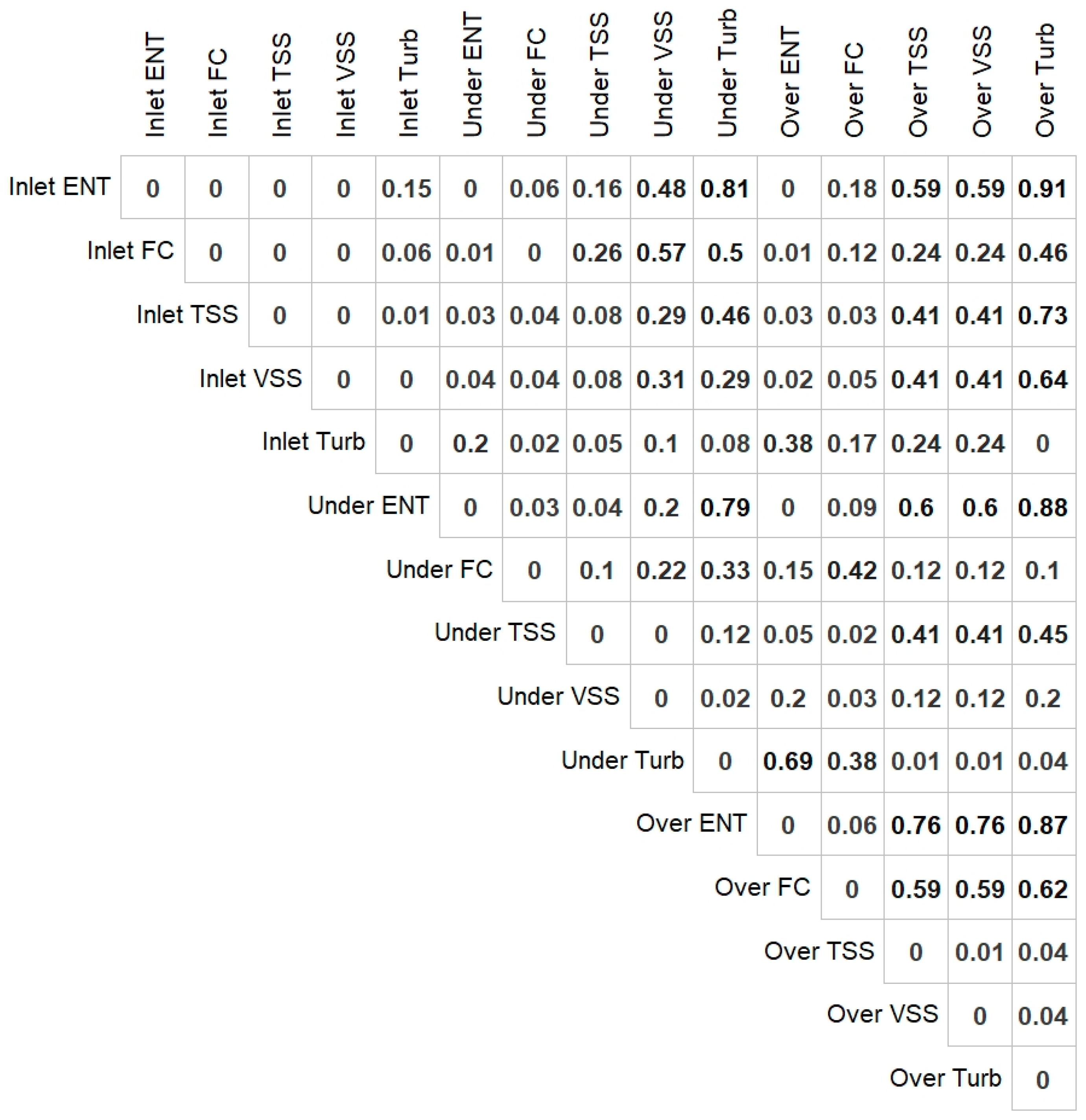
3.3. Statistically Significant Correlations

Several significant correlations were found to impact the bioswale’s performance (Figure 8) (p-value < 0.05 shows significance). The inflow concentration of enterococci and fecal coliform were positively correlated with both TSS and VSS. Thus, if sediment concentrations were high, one would likely observe higher enterococci and fecal coliform concentrations, which is logical since bacteria are often sediment-bound [84,85]. This potentially provides a framework for choosing locations to retrofit SCMs when targeting bacteria removal in a watershed: by simply measuring TSS or VSS concentrations, which is inherently less expensive and time consuming. Drainage areas that produce relatively higher sediment concentrations would appear to be good candidates for fecal coliform- and enterococcus-reducing SCMs, such as bioswales.

4. Summary and Conclusions

Concentrations for the five pollutants examined (turbidity, TSS, VSS, enterococci and fecal coliform) were uniformly lower in underdrain flow than in inflow. Greater than 55% removal was observed for FIB and greater than 85% removal for TSS, suggesting filtration is an effective removal mechanism for these pollutants. Overflow concentrations were similar to those from the underdrain; overflow was not treated to the same extent as drainage, but that overflowed occurred after the first flush, and therefore may have had lower bacterial concentrations. Fecal coliform outflow concentrations often met targets established by the USEPA [11] for recreational waters, but this was never the case for enterococci. A cause might be the markedly higher inflow concentrations measured for the latter indicator species. Turbidity targets were also met for both underdrain flow and overflow, but only underdrain outflow achieved TSS thresholds [75].

Synthesizing the results of this bioswale and comparing them to other SCMs indicates that the practice might be a popular tool. Bioswales fits within existing rights-of-way and water that infiltrates the media was measured to be cleaner than that of surface flow for common pollutants. This case study suggests that bioswales function should be more closely examined as a function of the ratio of watershed size to bioswale length, the impact of slope, drainage area properties, soil media type, etc. This will allow for design standards for bioswales to be crafted.

References

1. United Nations. World Urbanization Prospects: The 2014 Revision, Highlights; United Nations Department of Economic and Social Affairs, Population Division: New York, NY, USA, 2014; Available online: https://esa.un.org/unpd/wup/publications/files/wup2014-highlights.pdf (accessed on 1 October 2017).
2. Morisawa, M.; LaFlure, E. Hydraulic geometry, stream equilibrium and urbanization. In Adjustments of the Fluvial Systems, Proceedings of the 10th annual Geomorphology Symposium Series, Binghampton, New York, NY, USA, 21–22 September 1979; Rhodes, D.D., Williams, G.P., Eds.; Kendall/Hunt Publishing Co., Inc.: Dubuque, IA, USA, 1979. [Google Scholar]
3. Arnold, C.L.; Boison, P.J.; Patton, P.C. Sawmill Brook: An example of rapid geomorphic change related to urbanization. J. Geol. 1982, 90, 155–166. [Google Scholar] [CrossRef]
4. Bannerman, R.T.; Owens, D.W.; Dodds, R.B.; Hornewer, N.J. Sources of pollutants in Wisconsin stormwater. Water Sci. Technol. 1993, 28, 241–259. [Google Scholar]
5. Brabec, E.; Schulte, S.; Richards, P.L. Impervious surfaces and water quality: A review of current literature and its implications for watershed planning. J. Plan. Lit. 2002, 16, 499–514. [Google Scholar] [CrossRef]
6. Todeschinie, S. Hydrologic and Environmental Impacts of Imperviousness in an Industrial Catchment of Northern Italy. J. Hydrol. Eng. 2016, 21, 05016013. [Google Scholar] [CrossRef]
7. Thomson, N.R.; McBean, E.A.; Snodgrass, W.; Monstrenko, I.B. Highway stormwater runoff quality: Development of surrogate parameter relationships. Water Air Soil Pollut. 1997, 94, 307–347. [Google Scholar] [CrossRef]
8. Opher, T.; Friedler, E. Factors affection highway runoff quality. Urban Water J. 2010, 7, 155–172. [Google Scholar] [CrossRef]
9. Ingvertsen, S.T.; Cederkvist, K.; Régent, Y.; Sommer, H.; Magid, J.; Jensen, M.B. Assessment of existing roadside swales and engineered filter soil: I. Characterization and lifetime expectancy. J. Environ. Qual. 2012, 41, 1960–1969. [Google Scholar] [CrossRef] [PubMed]
10. U.S. Environmental Protection Agency (USEPA). National Summary of State Information; U.S. Environmental Protection Agency (USEPA): Washington, DC, USA, 2016. Available online: https://www.iaspub.epa.gov/waters10/attains_nation_cy.control (accessed on 5 June 2017).
11. U.S. Environmental Protection Agency (USEPA). 2012 Recreational Water Quality Criteria; EPA-820-F-12-061; USEPA Office of Water: Washington, DC, USA, 2012.
12. Mallin, M.A.; Williams, K.E.; Esham, E.C.; Lowe, R.P. Effect of human development on bacteriological water quality in coastal watersheds. Ecol. Appl. 2000, 10, 1047–1056. [Google Scholar] [CrossRef]
13. U.S. Environmental Protection Agency (USEPA). Protocol for Developing Pathogen TMDLs; EPA-841-R-00-002; USEPA Office of Water: Washington, DC, USA, 2001.
14. Stevik, T.K.; Aa, K.; Ausland, G.; Hanssen, J.F. Retention and removal of pathogenic bacteria in wastewater percolating through porous media: A review. Water Res. 2004, 38, 1355–1367. [Google Scholar] [CrossRef] [PubMed]
15. Arnone, R.D.; Walling, J.P. Waterborne pathogens in urban watersheds. J. Water Health 2007, 5, 149–162. [Google Scholar] [CrossRef] [PubMed]
16. Struck, S.D.; Selvakumar, A.; Borst, M. Prediction of Effluent Quality from Retention Ponds and Constructed Wetlands for Managing Bacterial Stressors in Storm-Water Runoff. J. Irrig. Drain. Eng. 2008, 134, 567–578. [Google Scholar] [CrossRef]
17. Weber-Shirk, M.L.; Dick, R.I. Physical-Chemical Mechanisms in Slow Sand Filters. J. Am. Water Works Assoc. 1997, 89, 87–100. [Google Scholar]
18. Rusciano, G.M.; Obropta, C.C. Bioretention column study: Fecal coliform and total suspended solids reductions. Trans. ASABE 2007, 50, 1261–1269. [Google Scholar] [CrossRef]
19. Sherer, B.M.; Miner, R.; Moore, J.A.; Buckhouse, J.C. Indicator bacterial survival in stream sediments. J. Environ. Qual. 1992, 21, 591–595. [Google Scholar] [CrossRef]
20. Mohanty, S.K.; Torkelson, A.A.; Dodd, H.; Nelson, K.L.; Boehm, A.B. Engineering Solutions to Improve the Removal of Fecal Indicator Bacteria by Bioinfiltration Systems during Intermittent Flow of Stormwater. Environ. Sci. Technol. 2013, 47, 10791–10798. [Google Scholar] [CrossRef] [PubMed]
21. Leclerc, H.; Mossel, D.A.A.; Edberg, S.C.; Struijk, C.B. Advances in the bacteriology of the coliform group: Their suitability as markers of microbial water safety. Annu. Rev. Microbiol. 2001, 55, 201–234. [Google Scholar] [CrossRef] [PubMed]
22. Savichtcheva, O.; Okabe, S. Alternative indicators of fecal pollution: Relations with pathogens and conventional indicators, current methodologies for direct pathogen monitoring and future application perspectives. Water Res. 2006, 40, 2463–2476. [Google Scholar] [CrossRef] [PubMed]
23. Pan, X.; Jones, K.D. Seasonal variation of fecal indicator bacteria in storm events within the US stormwater database. Water Sci. Technol. 2012, 65, 1076–1080. [Google Scholar] [CrossRef] [PubMed]
24. O’Neill, S.; Adhikari, A.R.; Gautam, M.R.; Acharya, K. Bacterial contamination due to point and nonpoint source pollution in a rapidly growing urban center in an arid region. Urban Water J. 2013, 10, 411–421. [Google Scholar] [CrossRef]
25. Hathaway, J.M.; Hunt, W.F.; Graves, A.K.; Wright, J.D. Field evaluation of bioretention indicator bacteria sequestration in Wilmington, NC. J. Environ. Eng. 2011, 137, 1103–1113. [Google Scholar] [CrossRef]
26. Li, Y.L.; Deletic, A.; Alcazar, L.; Bratieres, K.; Fletcher, T.D.; McCarthy, D.T. Removal of Clostridium perfringens, Escherichia coli, and F-RNA coliphanges by stormwater biofilters. Ecol. Eng. 2012, 49, 137–145. [Google Scholar] [CrossRef]
27. Rowny, J.G.; Stewart, J.R. Characterization of nonpoint source microbial contamination in an urbanizing watershed serving as a municipal water supply. Water Res. 2012, 46, 6143–6153. [Google Scholar] [CrossRef] [PubMed]
28. Fletcher, T.D.; Shuster, W.; Hunt, W.F.; Ashley, R.; Butler, D.; Arthur, S.; Trowsdale, S.; Barraud, S.; Semadeni-Davies, A.; Bertrand-Krajewski, J.L.; et al. SUDS, LID, BMPs, WSUD and more—The evolution and application of terminology surrounding urban drainage. Urban Water J. 2015, 12, 525–542. [Google Scholar] [CrossRef]
29. Rushton, B.T. Low-impact parking lot design reduces runoff and pollutants loads. J. Water Resour. Plan. Manag. 2001, 127, 172–179. [Google Scholar] [CrossRef]
30. Holman-Dodds, J.K.; Bradley, A.A.; Potter, K.W. Evaluation of hydrologic benefits of infiltration based urban storm water management. J. Am. Water Resour. Assoc. 2003, 39, 205–215. [Google Scholar] [CrossRef]
31. Hunt, W.F.; Davis, A.P.; Traver, R.G. Meeting hydrologic and water quality goals through targeted bioretention design. J. Environ. Eng. 2012, 138, 698–707. [Google Scholar] [CrossRef]
32. Barrett, M.E.; Wals, P.M.; Malina, J.F., Jr.; Charbeneau, R.J. Performance of vegetative controls for treating highway runoff. J. Environ. Eng. 1998, 124, 1121–1128. [Google Scholar] [CrossRef]
33. Davis, A.P.; Stagge, J.H.; Jamil, E.; Kim, H. Hydraulic performance of grass swales for managing highway runoff. Water Res. 2011, 46, 6775–6786. [Google Scholar] [CrossRef] [PubMed]
34. Deletic, A. Modelling of water and sediment transport over grassed areas. J. Hydrol. 2001, 248, 168–182. [Google Scholar] [CrossRef]
35. Bäckström, M. Sediment transport in grassed swales during simulated runoff events. Water Sci. Technol. 2002, 45, 41–49. [Google Scholar] [PubMed]
36. Barrett, M.E. Performance comparison of structural stormwater best management practices. Water Environ. Res. 2005, 77, 78–86. [Google Scholar] [CrossRef] [PubMed]
37. Ackerman, D.; Stein, E.D. Evaluating the effectiveness of best management practices using dynamic modeling. J. Environ. Eng. 2008, 134, 628–639. [Google Scholar] [CrossRef]
38. Knight, E.M.P.; Hunt, W.F., III; Winston, R.J. Side-by-side evaluation of four level spreader-vegetated filter strips and a swale in eastern North Carolina. J. Soil Water Conserv. 2013, 68, 60–72. [Google Scholar] [CrossRef]
39. Stagge, J.H.; Davis, A.P.; Jamil, E.; Kim, H. Performance of grass swales for improving water quality from highway runoff. Water Res. 2012, 46, 6731–6742. [Google Scholar] [CrossRef] [PubMed]
40. Yu, S.L.; Kuo, J.T.; Fassman, E.A.; Pan, H. Field test of grassed-swale performance in removing runoff pollution. J. Water Resour. Plan. Manag. 2001, 127, 168–171. [Google Scholar] [CrossRef]
41. Lucke, T.; Mohamed, M.A.K.; Tindale, N. Pollutant removal and hydraulic retention performance of field grassed swales during runoff simulation experiments. Water 2014, 6, 1887–1904. [Google Scholar] [CrossRef]
42. Davis, A.P.; Hunt, W.F.; Traver, R.G.; Clar, M. Bioretention technology: Overview of current practice and future needs. J. Environ. Eng. 2009, 135, 109–117. [Google Scholar] [CrossRef]
43. Christianson, R.D.; Barfield, B.J.; Hayes, J.C.; Gasem, K.; Brown, G.O. Modeling effectiveness of bioretention cells for control of stormwater quantity and quality. In Critical Transitions in Water and Environmental Resources Management, Proceedings of the 2004 World Water and Environmental Resources Congress, Salt Lake City, UT, USA, 27 June –1 July 2004; American Society of Civil Engineers: Reston, VA, USA, 2004. [Google Scholar]
44. Davis, A.P.; Shokouhian, M.; Sharma, H.; Minami, C. Laboratory study of biological retention for urban stormwater management. Water Environ. Res. 2001, 73, 5–14. [Google Scholar] [CrossRef] [PubMed]
45. Hunt, W.F.; Jarrett, A.R.; Smith, J.T.; Sharkey, L.J. Evaluating bioretention hydrology and nutrient removal at three field sites in North Carolina. J. Irrig. Drain. Eng. 2006, 132, 600–608. [Google Scholar] [CrossRef]
46. Garbrecht, K.; Fox, G.A.; Guzman, J.A.; Alexander, D. E. coli transport through soil columns: Implications for bioretention cell removal efficiency. Trans. ASABE 2009, 52, 481–486. [Google Scholar] [CrossRef]
47. Hunt, W.F.; Smith, J.T.; Jadlocki, S.J.; Hathaway, J.M.; Eubanks, P.R. Pollutant removal and peak flow mitigation by a bioretention cell in urban Charlotte, N.C. J. Environ. Eng. 2008, 134, 403–408. [Google Scholar] [CrossRef]
48. Hathaway, J.M.; Hunt, W.F.; Jadlocki, S. Indicator bacteria removal in stormwater best management practices in Charlotte, North Carolina. J. Environ. Eng. 2009, 135, 1275–1285. [Google Scholar] [CrossRef]
49. Zinger, Y.; Deletic, A.; Fletcher, T.D.; Breen, P.; Wong, T. A Dual-Mode Biofilter System: Case Study in Kfar Sava, Israel. In Proceedings of the 12th International Conference on Urban Drainage, Porto Alegre, Brazil, 11–16 September 2011. [Google Scholar]
50. Zhang, L.; Seagren, E.A.; Davis, A.P.; Karns, J.S. Effects of temperature on bacterial transport and destruction in bioretention media: Field and laboratory evaluations. Water Environ. Res. 2012, 84, 485–496. [Google Scholar] [CrossRef] [PubMed]
51. McLaughlin, J. NYC bioswales pilot project improves stormwater management. Clear Waters 2012, 2012, 20–23. [Google Scholar]
52. Xiao, Q.; McPherson, E.G. Testing a Bioswale to Treat and Reduce Parking Lot Runoff. Center for Urban Forest Research, University of California-Davis, 2009. Available online: https://www.fs.fed.us/psw/topics/urban_forestry/products/psw_cufr761_P47ReportLRes_AC.pdf (accessed on 14 April 2017).
53. Anderson, B.S.; Phillips, B.M.; Voorhees, J.P.; Siegler, K.; Tjeerdema, R. Bioswales reduce contaminants associated with toxicity in urban storm water. Environ. Toxicol. Chem. 2016, 35, 3124–3134. [Google Scholar] [CrossRef] [PubMed]
54. Stantec. Lockwoods Folly River Local Watershed Plan Preliminary Findings Report for North Carolina Ecosystem Enhancement Program; Stantec Consulting Services Inc.: Raleigh, NC, USA, 2006. Available online: https://www.ncdeq.gov (accessed on 3 May 2017).
55. U.S. Environmental Protection Agency (USEPA). North Carolina Water Quality Assessment Report. 2014. Available online: https://iaspub.epa.gov/waters10/attains_state.control?p_state=NC (accessed on 3 May 2017).
56. U.S. Census Bureau. Resident Population Estimates for the 100 Fastest Growing U.S. Counties with 10,000 or More Population in 2010: 1 April 2010 to 1 July 2016. U.S. Census Bureau Population Division: Washington, DC, USA, 2017. Available online: https://factfinder.census.gov (accessed on 1 October 2017).
57. North Carolina Department of Transportation (NCDOT). Standard Specifications—16 Erosion Control and Roadside Development. North Carolina Department of Transportation: Raleigh, NC, USA, 2012. Available online: https://connect.ncdot.gov/resources/Specifications/Pages/2012StandSpecsMan.aspx?Order=SM-16-1610 (accessed on 15 November 2017).
58. North Carolina Department of Transportation. Division 10 Materials. North Carolina Department of Transportation: Raleigh, NC, USA, 2016. Available online: https://connect.ncdot.gov/resources/specifications/2006%20specifications%20books/10.%20materials.pdf (accessed on 15 November 2017).
59. Brown, R.A.; Hunt, W.F. Underdrain configuration to enhance bioretention exfiltration to reduce pollutant loads. J. Environ. Eng. 2011, 137, 1082–1091. [Google Scholar] [CrossRef]
60. Winston, R.J.; Dorsey, J.D.; Hunt, W.F. Quantifying volume reduction and peak flow mitigation for three bioretention cells in clay soils in northeast Ohio. Sci. Total Environ. 2016, 553, 83–95. [Google Scholar] [CrossRef] [PubMed]
61. U.S. Environmental Protection Agency (USEPA). NPDES Storm Water Sampling Guidance Document; EPA 833-B-92-002; USEPA Office of Water: Washington, DC, USA, 1992.
62. American Public Health Association (APHA). Conductivity; SM 2510b-97; APHA: Washington, DC, USA, 1997. [Google Scholar]
63. American Public Health Association (APHA). Turbidity; SM 2130b-01; APHA: Washington, DC, USA, 2001. [Google Scholar]
64. American Public Health Association (APHA). Total Suspended Solids; SM 2540d-97; APHA: Washington, DC, USA, 1997. [Google Scholar]
65. American Public Health Association (APHA). Fixed and Volatile Solids; SM 2540e-97; APHA: Washington, DC, USA, 1997. [Google Scholar]
66. American Public Health Association (APHA). Fecal Coliform Procedure; SM 9221e-99; APHA: Washington, DC, USA, 1999. [Google Scholar]
67. ASTM. Standard Test Method for Enterococci in Water Using Enterolert; ASTM D6503-14; ASTM: West Conshohocken, PA, USA, 2014. [Google Scholar]
68. R Core Team. R: A Language and Environment for Statistical Computing; R Foundation for Statistical Computing: Vienna, Austria, 2013; ISBN 3-900051-07-0. [Google Scholar]
69. U.S. Environmental Protection Agency (USEPA). Urban Stormwater BMP Performance Monitoring; EPA-821-B-02-001; USEPA Office of Water: Washington, DC, USA, 2002.
70. Burton, G.A.; Pitt, R.E. Stormwater Effects Handbook: A Toolbox for Watershed Managers, Scientists, and Engineers; CRC: Boca Raton, FL, USA, 2002. [Google Scholar]
71. Davis, A.P.; Shokouhian, M.; Sharma, H.; Minami, C.; Winogradoff, D. Water quality improvement through bioretention: Lead, copper, and zinc removal. Water Environ. Res. 2003, 75, 73–82. [Google Scholar] [CrossRef] [PubMed]
72. Davis, A.P.; Shokouhian, M.; Sharma, H.; Minami, C. Water quality improvement through bioretention media: Nitrogen and phosphorus removal. Water Environ. Res. 2006, 78, 284–293. [Google Scholar] [CrossRef] [PubMed]
73. Deletic, A.; Fletcher, T.D. Performance of grass filters used for stormwater treatment—A field and modelling study. J. Hydrol. 2006, 317, 261–275. [Google Scholar] [CrossRef]
74. Winston, R.J.; Hunt, W.F.; Kennedy, S.G.; Wright, J.D.; Lauffer, M.S. Field evaluation of storm-water control measures for highway runoff treatment. J. Environ. Eng. 2012, 138, 101–111. [Google Scholar] [CrossRef]
75. North Carolina Department of Environmental Quality (NCDEQ). Surface Waters and Wetland Standards; 15A NCAC 2B; NCDEQ Division of Water Quality: Raleigh, NC, USA, 2007.
76. Barrett, M.E. Performance, cost, and maintenance requirements of Austin sand filters. J. Water Resour. Plan. Manag. 2003, 129, 234–242. [Google Scholar] [CrossRef]
77. Hathaway, J.M.; Hunt, W.F. Evaluation of first flush for indicator bacteria for total suspended solids in urban stormwater runoff. Water Air Soil Pollut. 2011, 217, 135–147. [Google Scholar] [CrossRef]
78. Hathaway, J.M.; Hunt, W.F. Indicator Bacteria Performance of Stormwater Control Measures in Wilmington, NC. J. Irrig. Drain. Eng. 2012, 138, 185–197. [Google Scholar] [CrossRef]
79. Passeport, E.; Hunt, W.F.; Line, D.E.; Smith, R.A.; Brown, R.A. Field study of the ability of two grassed bioretention cells to reduce storm-water runoff pollution. J. Irrig. Drain. Eng. 2009, 135, 505–510. [Google Scholar] [CrossRef]
80. Davis, A.P. Field Performance of Bioretention: Water Quality. Environ. Eng. Sci. 2007, 24, 1048–1064. [Google Scholar] [CrossRef]
81. Davies, C.M.; Bavor, H.J. The fate of stormwater-associated bacteria in constructed wetland and water pollution control pond systems. J. Appl. Microbiol. 2000, 89, 349–360. [Google Scholar] [CrossRef] [PubMed]
82. Krometis, L.H.; Drummey, P.N.; Characklis, G.W.; Sobsey, M.D. Impact of microbial partitioning on wet retention pond effectiveness. J. Environ. Eng. 2009, 135, 758–767. [Google Scholar] [CrossRef]
83. Mallin, M.A.; Ensign, S.H.; Wheeler, T.L.; Mayes, D.B. Pollutant removal efficacy of three wet detention ponds. J. Environ. Qual. 2002, 31, 654–660. [Google Scholar] [CrossRef] [PubMed]
84. Characklis, G.W.; Dilts, M.J.; Simmons, O.D., III; Likirdopulos, C.A.; Krometis, L.-A.H.; Sobsey, M.D. Microbial partitioning to settleable particles in stormwater. Water Res. 2005, 39, 1773–1782. [Google Scholar] [CrossRef] [PubMed]
85. Krometis, L.-A.H.; Characklis, G.W.; Simmons, O.D., III; Dilts, M.J.; Likirdopulos, C.A.; Sobsey, M.D. Intra-storm variability in microbial partitioning and microbial loading rates. Water Res. 2007, 41, 506–516. [Google Scholar] [CrossRef] [PubMed]
Figure 1. Watershed, grassed shoulder, and concrete-lined channel leading to the forebay of the bioswale.
Water 10 00134 g001
Figure 2. Horizontal cross-section of the underdrained portion (flow going into page). Note-not to scale.
Water 10 00134 g002
Figure 3. Full structure longitudinal cross-section. Note: not to scale.
Water 10 00134 g003
Figure 4. Bioswale outlet structure, with the upstream grate housing the underdrain monitoring and the downstream grate housing the overflow monitoring. The completed bioswale is present in the background.
Water 10 00134 g004
Figure 5. (a) Sixty-degree v-notch weir installed to measure drainage from the underdrain and pond water for sampling (flow direction from background to foreground); (b) Ninety-degree v-notch weir installed to measure overflow/bypass with a baffle (center) to still flow for sampling (flow direction from left to right).
Water 10 00134 g005
Figure 6. Enterococci probability plot with water quality standard of 35 MPN/100 mL.
Water 10 00134 g006
Figure 7. Fecal coliform probability plot with water quality standard of 200 MPN/100 mL.
Water 10 00134 g007
Figure 8. Kendall’s Tau p-value correlation matrix for all pollutants (a = 0.05).
Water 10 00134 g008